Case Selection

LASSO scenarios focus on specific meteorological regimes, and thus require careful selection of case dates to be simulated. A balance is struck between the number of cases, size of the modeling configuration, and available resources. For LASSO-CACTI, a two-stage process was employed to scan a larger number of case dates with coarser grid spacing followed by targeted simulations at LES scale.

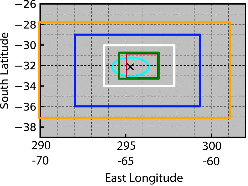
Figure 2 Illustration of WRF nested domains relative to the AMF location (the ‘X’) and ARM C-Band scanning domain (cyan oval). The oval is the projection-distorted ‘circular’ domain for the ARM C Band radar products, which have a ~100-km radius. Note that a ridge blocks the radar signal approximately westward of 295°E (65°W) so that the evaluation region is limited to the red box. The outer colored boxes indicate the four nested WRF domains.

The selection process consisted of the following steps:

1. A list of candidate dates was obtained from Adam Varble, the CACTI PI. The list considered factors such as convection cases coinciding with data/instrument availability.

2. Animations of VISST IR satellite data were then inspected for the occurrence of convective initiation and upscale growth occurring within the CSAPR2 observational domain. Cases were not considered when convection only occurred outside of the CSAPR2 domain or when initiation occurred outside of this domain and then advected into it, as the upscale growth would not be observable by ARM instrumentation, and adding value to the ARM measurements is a primary goal of LASSO. The extents of the WRF domains in relation to the region visible to the C-band radar are shown in Figure 2.

3. A range of convective behavior was sought for which CAPE was used as an index to verify that a sampling of the range had been achieved for the chosen dates. CAPE values (J kg-1) were calculated using both the most unstable layer (MU) and the mixed layer (ML) methodologies. Selections through this stage produced 20 case dates, which we refer to as the “mesoscale cases,” with the list of mesoscale case dates shown in Table 2.

4. A 33-member ensemble of mesoscale simulations were conducted (∆x=2.5-km grid spacing) for each mesoscale case day. The ensemble members correspond to different large-scale forcings from ERA5 (1 member), FNL (1 member), ERA5-EDA (10 members), and GEFS (21 members) as described in the Initial and Boundary Condition section. Case days with poor ensemble performance were assigned lower priority as the large-scale conditions might not be adequately captured in the available forcings. Some questionable case days were still retained, as it was possible that the LES resolution (∆x=100 m) might improve dynamical features unresolved at 2.5 km that could improve the simulation.

This selection process resulted in nine potentially viable LES case dates, listed in Table 2 as cases that include a letter alongside the case number. These dates have dedicated pages with more extensive descriptions accessed by the links in the table. The descriptions include a snapshot of the satellite IR brightness temperature (at 11.2 μm) aimed at illustrating a distinguishing phase of the development. The remaining cases with only mesoscale ensembles include a short description directly in Table 2.

Note that the black X in Figure 2 indicates the location of the AMF site and the white box indicates the domain used for the Δx=500-m grid (domain 3) in the LES simulations.

Satellite-based animations of brightness temperature for all days are available via the Bundle Browser. Look in the table of simulations for each case date under the “Sim. Tb” column to access animations for the simulations, and look in the “Observation Summary” pages of the case dates for the observed brightness temperature animations.

Table 2 Case dates selected for LASSO-CACTI. Lettered cases in bold are simulated at both mesoscale and LES scales. Days with only a number are only simulated for the mesoscale ensemble.

Case	Date	Description
1	2018-10-26	Propagating, isolated system Daytime region remains clear until 20 UTC when a small, isolated system develops far to the southwest of the AMF that rapidly transverses the region to dissipate over the AMF by 23:30 UTC. At 16 UTC MUCAPE=1,155, MLCAPE=62 J kg-1.
2	2018-11-04	Single, fleeting system Daytime region remains clear until 18 UTC when a small, isolated system develops over the AMF that propagates away and dissipates by 17:15 UTC. At 18 UTC MUCAPE=2,860, MLCAPE=1,061 J kg-1. A G-1 flight day.
3	2018-11-05	Discrete MCS Propagation A cell initiates slightly behind the ridgeline just north of the AMF at 14:15 UTC and develops in isolation there until moving away by 18:30 UTC. At 15 UTC MUCAPE=1,007, MLCAPE=232 J kg-1. A RELAMPAGO mission day. This case is highlighted in Lombardo and Kumjian [2022] for discrete MCS propagation.
4	2018-11-06	Deep convection initiates from behind the ridgeline Deep convection initiates behind the ridgeline at 18:30 UTC and grows over the AMF before advecting northwest and dissipating at 21:30. At 15 UTC MUCAPE=1,753, MLCAPE=219 J kg-1. A G-1 flight day and RELAMPAGO mission day.
5	2018-11-10	Fleeting, rapidly developed MCS Convective initiation occurs over the AMF at 19 UTC that rapidly develops into an MCS while moving out of the region by 20 UTC. At 15 UTC MUCAPE=4,322, MLCAPE=2,200 J kg-1. A G-1 flight day and RELAMPAGO mission day.
6	2018-11-21	Orographic congestus Orographic congestus develops by midafternoon but does not initiate into anything intense. At 18 UTC MUCAPE=2,882, MLCAPE=2,249 J kg-1. A G-1 flight day and RELAMPAGO mission day.
7, A	2018-11-29	Convective initiation with halted upscale growth Details
8	2018-11-30	Convective initiation and merging near the site Convective initiation just south of the AMF at 19 UTC that develops while merging with a system coming from the southwest behind the ridgeline by 21 UTC. At 18 UTC MUCAPE=2,177, MLCAPE=938 J kg-1. A RELAMPAGO mission day.
9, B	2018-12-04	Moderately sized system develops north of the AMF Details
10, C	2018-12-05	Three cells initiate and grow near the AMF into small sizes Details
11, D	2018-12-19	Convective initiation and growth over the AMF within a complicated background field Details
12, E	2019-01-22	Two intense systems develop next to each other Details
13, F	2019-01-23	An intense, organized system is formed from multi-cell interactions Details
14, G	2019-01-25	Monster mesoscale convective system Details
15, H	2019-01-29	An intense case like January 22nd (12, E) that has similar CAPE but less shear Details
16	2019-01-31	Convective streak initiates behind the ridgeline A streak of intense convection initiates at 17:30 northwest of the AMF behind the ridgeline, followed by intense convection entering the region from behind the ridgeline by 19 UTC. At 18 UTC MUCAPE=2,833, MLCAPE=880 J kg-1.
17, I	2019-02-08	Many convective initiations over and around the AMF Details
18	2019-02-23	Pop-up cells near the AMF A few small, fleeting convective cells initiate over the AMF starting 19:30 and advect out of the region. At 18 UTC MUCAPE=1,163, MLCAPE=723 J kg-1. The CSAPR2 scanning cross-wind only.
19	2019-03-14	Isolated streak of intense convection An isolated cell initiates just north of the AMF at 17 UTC and develops into a streak of intense convection that dissipates by 22 UTC. At 18 UTC MUCAPE=2,608, MLCAPE=1,659 J kg-1. The CSAPR2 scanning cross-wind only.
20	2019-03-15	Large convective system advects over site, initiation not observed A large convective system initiates and develops to the southwest of the AMF behind the ridgeline before advecting over the AMF starting 11 UTC. At 12 UTC MUCAPE=579, MLCAPE=470 J kg-1. The CSAPR2 scanning cross-wind only.