Observations and Skill Scores
Simulation quality is assessed through comparisons with regionally representative observations within the vicinity of the AMF and is quantified using skill scores. The skill scores monotonically increase with improved skill from 0 to 1, where 0 indicates no skill and 1 indicates perfect agreement in terms of the metric. Users can use these skill scores to ascertain general model behavior for their application of interest when sorting through the available simulations. More detailed comparisons with observations are left to users to perform based on their particular research needs. The observations and skill scores are described below.
This section of the documentation focuses on how the skill scores and diagnostics are calculated. The skill scores and their plots are accessible via the LASSO-CACTI Bundle Browser. Specifics on where in the Browser to go are described in the Bundle Browser section.
Brightness Temperature for Convective Area Development
The time evolution of simulated convective areas within the region are assessed using geostationary satellite observations of brightness temperature (Tb), which is the outgoing infrared energy expressed in terms of the temperature of an equivalent black body emitter. The regions of deep convective activity in the simulations and satellite data are obtained using a mask for an “anvil” Tb threshold of <240 K [Laing and Fritsch, 1993]. This Tb threshold is associated with well-developed anvils that are sufficiently opaque to prevent the direct transmission of infrared energy from the surface thereby providing an effective temperature of the cloud (and not a mixture of cloud emission plus transmitted radiation from the surface). Observations are from the GOES-16 11.2-μm narrowband window channel, obtained from NASA LaRC Satellite ClOud and Radiation Property retrieval System (SatCORPS), that have been parallax-corrected. The Tb for the simulations is determined as the atmospheric temperature at which the infrared optical depth reaches two when integrating downwards from the top model level (equivalent to an absorption optical depth of one), which is where peak sensitivity to outgoing radiation occurs [Vogelmann and Ackerman, 1995] and the level that is interpreted as the effective emission level of the IR radiation. (We note that a detailed study of the emission level optical depth found a range of 0–2 with a most likely value of 0.72 [Wang et al., 2014]. The difference from the value of two used here will underestimate the masked area in the simulations but likely not significantly because of the tight gradient in optical depth at the tops of well-developed anvils.)
The binary masking for the Tb threshold <240 K is done in the simulations and observations at 15-minute intervals, corresponding to the available frequency of the satellite data, and the skill scores are computed for each interval for the innermost D4 region (c.f., Figure 12).
The fidelity of the simulated deep convective regions for all mesoscale and LES runs is quantified using the Critical Success Index (CSI, which we denote as SCSI) and Frequency Bias (FB) [Gilbert, 1884, Mesinger and Black, 1992, Schaefer, 1990]. The CSI (also known as the “Threat Score”) is given by
and the Frequency Bias is
where,
\(N_H\) = number of hits (correctly forecast events)
\(N_{FA}\) = number of false alarms (incorrectly forecast non-events)
\(N_M\) = number of misses (incorrectly forecast events)
While the range of SCSI is [0,1], for FB it is [0, \(\infty\)] with perfect agreement at 1. To cast the FB in a form that conforms to a range [0,1], we create the Frequency Bias Skill, SFB, score by
noting that the most important thing for our application is how close the simulation is to 1, not the details of skill depreciation far from 1 (e.g., near infinity). Finally, for convenience, we combine the SCSI and SFB scores into a single skill score termed the Net Skill, SNet,
which, like its parent skill scores, has a range of [0,1] with perfect agreement at 1. All three skill scores—SCSI, SFB, SNet—are made available. Since some of the scores are used for multiple variables, we add the specific variable in parentheses when the context does not make the association clear, e.g., SFB(Tb).
The location of the convection is best characterized by SCSI(Tb) and the total area by SFB(Tb).
Examples of the skill scores are given in Figure 14 to Figure 17.
For the most basic level, an example of masking and skill scores is given in Figure 14. Like images are available every 15 minutes after removing the initial 6-hour spin-up period. The image contains the skill scores at the left, and display going to the right the masked regions from the observations, simulation, and their intersection. Scrolling through the plots shows the time evolution of the skill scores for the simulation to enable users to assess the simulation quality.
The skill scores for the whole simulation are aggregated into a single plot to show their time-evolution, as demonstrated in Figure 15, which shows a rapid increase in skill scores after convection initiates at 16 UTC (by construction, the skill scores are 0 when convection is absent and no value is provided when observations are unavailable). These values are also made available in comma-separated values (CSV) files (e.g., see Figure 16) for a closer inspection of periods of interest.
To facilitate comparison of all mesoscale simulations for a given case day, averages of the SCSI(Tb) and SFB(Tb) scores are separately computed for a post-convective initiation period, taken to be 15–24 UTC, and presented as a scatter plot. Figure 17 shows the results for the case day of 4 December 2018 where each point represents a single simulation and the best overall simulations are closest to (1,1). Note that this is an average performance while, for example, one might be more interested in the performance at the beginning of the simulation during the convective initiation and upscale growth without the influence on the skill scores of the developed convection later in the simulation. To identify periods of interest, users are referred to CSV files that contain the detailed time-evolution of the skill scores (e.g., Figure 16).
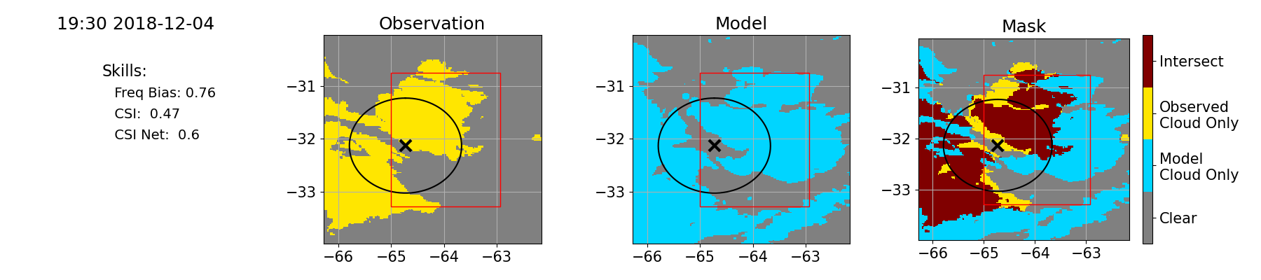
Figure 14 An example of masking and skill scores for the 4 December 2018 case at 19:30 UTC for a mesoscale run that used the GEFS04 forcing and Morrison microphysics. The first two images show the convective regions from masking for the “anvil” Tb threshold of <240 K, respectively for observations (yellow) and the simulation (blue), and the third plot shows model-observation intersection (burgundy). The region displayed is the D3 domain (c.f., Figure 12) and the skill scores are computed only for the D4 domain indicated by the red box. The skill scores are given at the left for the Frequency Bias Skill (SFB(Tb)), CSI (SCSI(Tb)), and Net Tb Skill (SNet(Tb)). For reference, the location of the AMF is indicated by the ‘X’ and the oval indicates the unobstructed, projection-altered scanning radius of the ARM precipitation radar.
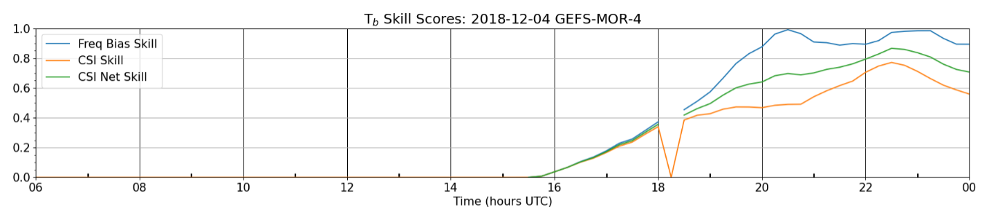
Figure 15 An example of the time-evolution of the skill scores for the whole simulation in Figure 14, which is for the 4 December 2018 case for the GEFS4 forcing and Morrison microphysics. The spike at 18:15 UTC is due to a data gap.
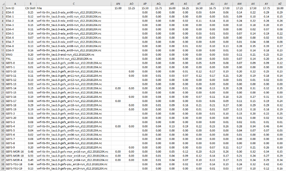
Figure 16 Example of the TbCSI CSV file contents displayed in Excel. This file shows the SCSI(Tb) skill values for the ensemble of mesoscale simulations run for 4 December 2018 (the SFB(Tb) and SNet(Tb) values are available in separate files). Reading from the left: Sim ID, indicating the mesoscale ensemble member used and any variations from the default for the microphysics or PBL scheme; SCSI(Tb), the average SCSI(Tb) for the period 15–24 UTC; and File, the original input file name for bookkeeping. The remaining columns show the SCSI(Tb) values for each 15-minute period for the UTC given at the top. For conciseness, this example hides the columns D to AM for the pre-convection period from 6.00 to 14.75 UTC and only shows a subsample of times during 15.00–18.00 UTC.
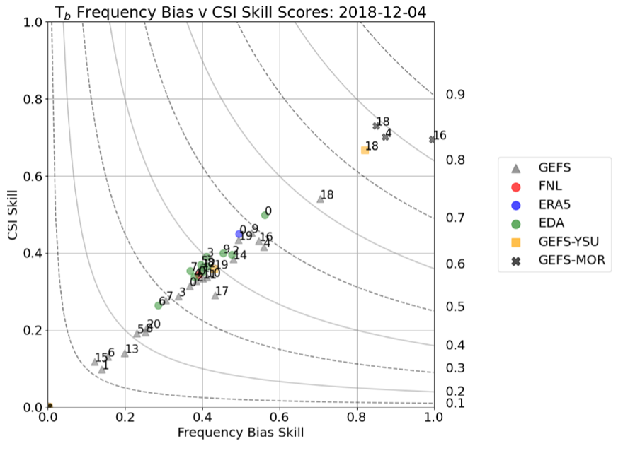
Figure 17 Scatter plot of the average CSI Skill (SCSI(Tb)) and Frequency Bias Skill (SFB(Tb)) scores for the post-initiation period during 15–24 UTC. The legend indicates the ensemble source of the forcing and the numbers in the plots indicate the ensemble member number. The contours indicate isopleths of Net Skill (SNet(Tb)), labeled at the right-hand y axis.
Echo-Top Heights for Local Convective Intensity
The simulated local convective intensity is assessed using radar echo-top height (ETH) for 20 dBZ, which generally indicates falling precipitation. Observations are from the second-generation C-Band Scanning ARM Precipitation Radar (CSAPR2) that were calibrated using onsite engineering measurements and cross-instrument comparisons [Hardin et al., 2020a] and processed using the Taranis package [Hardin et al., 2020b]. Data are used from within a scanning radius of 110 km from the site that are east of approximately −65°W longitude where a ridgeline blocks the beam. The simulated 20 dBZ level is obtained directly from the WRF output files for the region corresponding to the D4 domain east of −65°W longitude. The altitude of the 20 dBZ returns (above the radar at ground level) are determined in the observations and simulations at 15-minute intervals and averaged for comparison. Figure 18 shows an example comparison for the mesoscale ensemble run for 25 January 2019.
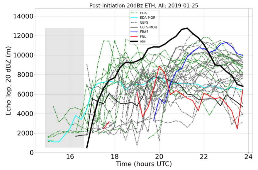
Figure 18 Domain-average heights of the ETH at 20 dBZ for 25 January 2019 for the post-initiation period during 15–24 UTC. The heavy black line is from the CSAPR2 observations and the other lines are from the mesoscale ensemble members. The gray shading indicates a period when observations are not available.
Model performance of ETH is quantified by a methodology that was successfully used for the evaluation of time series data in the LASSO shallow convection scenario—see Section 4.2 of Gustafson et al. [2020]. Performance is quantified using two skill scores: one characterizes the agreement of the variation/shape of the time series and the other characterizes its mean. The Taylor Skill score (Equation 4 in Taylor [2001]), ST, is used for the variation/shape of the distribution, as
where \(\sigma _r\) is the normalized standard deviation given by model root mean square (RMS) divided by the observed RMS, R is the correlation coefficient, and R0 is the maximum correlation attainable, which we set to 1. Thus, if the correlation coefficient and normalized standard deviation are 1, the Taylor Skill is 1. When applying the Taylor Skill score to a specific variable, we add the variable name, as done for the other skill scores, e.g., ST(ETH).
However, the Taylor Skill alone cannot characterize the time series performance because it does not include information regarding the mean. This information is included using a skill score for the relative mean, SRM, where the ratio, x, of the model mean divided by the observed mean is used in place of FB in Equation (3). This produces a skill score with the range [0,1] and is symmetric around one. As before, it is designed to quantify the relative difference from 1 and will yield the same value if the model underestimates or overestimates by the same factor. For example, two relative means that are different from observations by a factor of 2 on the low and high side, i.e., relative means of 0.5 and 2.0, would have the same skill score of 0.5 implying comparable performance relative to 1.
Finally, like the Net Tb Skill score (SNet(Tb)), we find it useful to combine the ST(ETH) and SRM(ETH) scores into a single Net ETH Skill Score, SNet(ETH). It is computed using Equation (4) where the CSI-related variables are replaced by ST(ETH) and SRM(ETH).
The focus of the skill scores is on the post-convective initiation period, taken to be 15–24 UTC, but we also characterize the performance of the pre-initiation period during 6–15 UTC following model spin-up. The Taylor Skill approach could not be used for this earlier period due to the frequent absence of ETH returns and flat distributions. Instead, we computed the root mean square difference (RMSD) over the period for the simulation, where the lowest values indicate the best performance.
An example of the Taylor-based skill scores is given in Figure 19 for the mesoscale ensembles shown in Figure 18, where the Taylor Skill (ST(ETH)) is plotted versus the Relative Mean Skill (SRM(ETH)). These values and the time series of domain-averaged ETH values are also made available in CSV files for a closer inspection of periods of interest (see Figure 20). An example of the pre-initiation RMSDs for the ensemble is given in Figure 21.
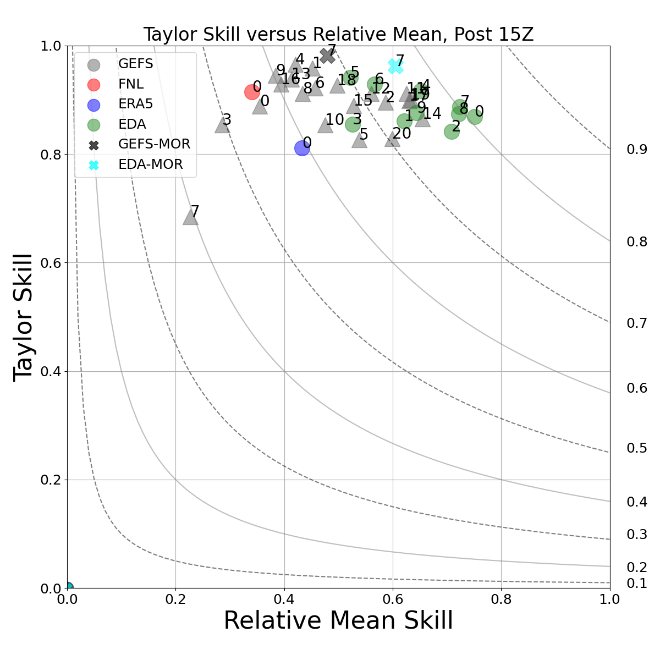
Figure 19 Scatter plot of the ETH scores for Relative Mean Skill (SRM) and Taylor Skill (ST) over the post-initiation period during 15–24 UTC for the mesoscale ensemble members from 25 January 2019. The legend indicates the ensemble source of the forcing and the numbers in the plots indicate the ensemble number. The contours indicate isopleths of Net ETH Skill (SNet(ETH)), labeled at the right-hand y axis.
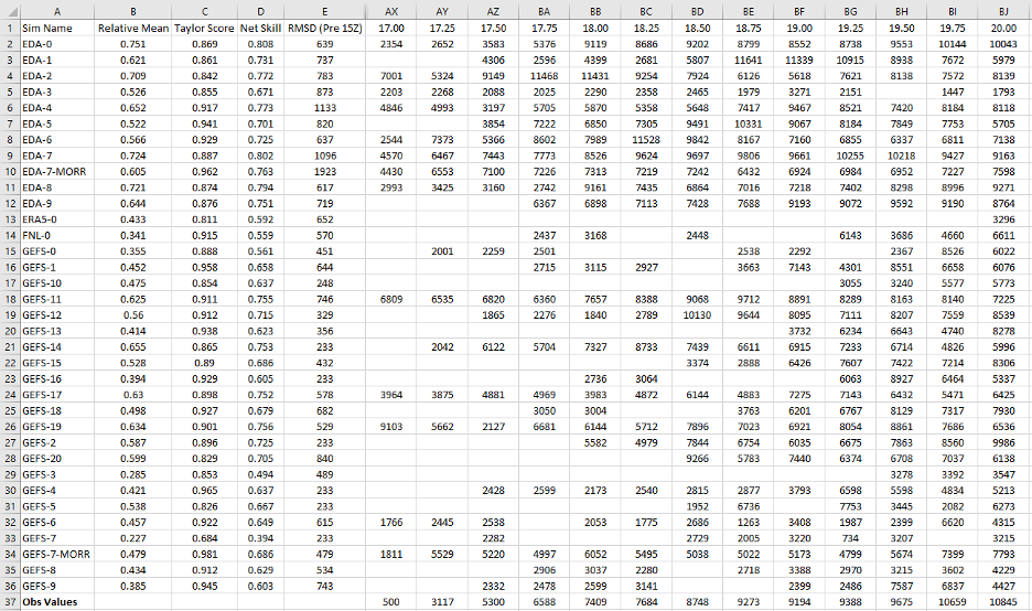
Figure 20 Example of the ETH CSV file contents displayed in Excel for the ensemble of mesoscale simulations run for 25 January 2019. Reading from the left: Sim ID, indicating the mesoscale ensemble member used and any variations from the default for the microphysics or PBL scheme with the observed value (‘Obs’) in the last row; Relative Mean Skill for ETH (SRM(ETH)); Taylor Score (ST(ETH)), the Taylor ETH Skill score; Net Skill, the Net ETH Skill (SNet(ETH)) score; and RMSD (Pre 15 UTC), the RMSD computed over the period 6–15 UTC characterizing simulation quality for the pre-initiation period. The remaining columns contain the domain-averaged ETH for each 15-minute period for the UTC given at the top, e.g., 17.00–20.00 UTC, with columns F to AX for the pre-convective initiation period hidden in this example.
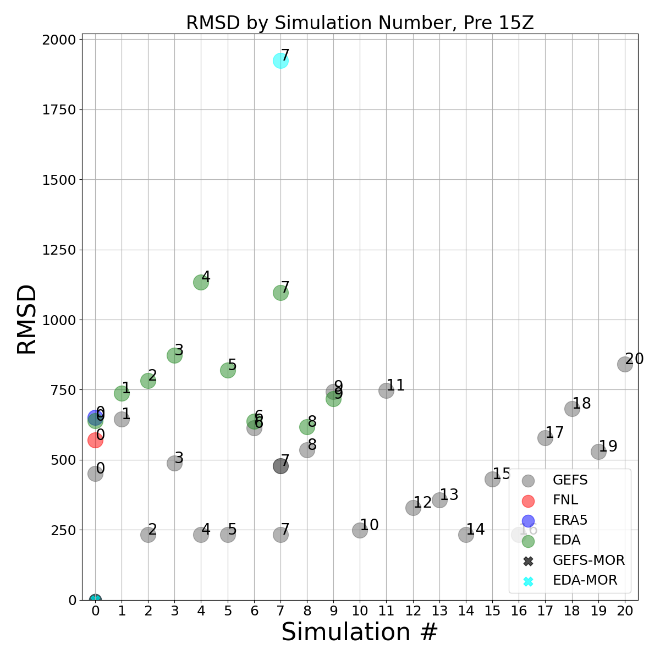
Figure 21 Plot of the RMSD for the pre-convective initiation period for the ensemble of mesoscale simulations run for 25 January 2019. The RMSD calculation neglects model spin up prior to 6 UTC and is computed over the period 6–15 UTC. The lower the value, the better the simulated pre-initiation period.
Regional Surface Rain Rate
Simulated surface rain rates are assessed using radar-derived estimates from the CSAPR2 data as processed by the Taranis package. We note that this assessment carries more uncertainty than for the Tb and ETH skill scores due to the combination of the limited area of the storm system sampled by the CSAPR2 scanning radius, the highly variable and spotty nature of precipitation, and the observed 15-minute temporal resolution that is coarse relative to the temporal variations in the phenomena. Nevertheless, surface rain rate is valuable in conveying the end-of-the-line outcome of all storm processes in an easily understood variable.
For the analyses, the observed and model domains are the same as used for ETH. Comparisons are made for region-averaged rain rate at hourly resolution. Observations are instantaneous values (i.e., based on one full plan position indicator [PPI] radar scan) sampled every 15 minutes that are averaged spatially over the domain and assumed to be constant for each 15-minute accumulation period. Simulated values are obtained from the accumulated surface precipitation every 15 minutes and processed into an hourly average estimate of rain rate for the region. All rain analyses are done using the 2.5-km grid spacing from the map of domain 2, with regridding to this grid done with the xESMF Python package and its conservative regridding methodology [Zhuang et al., 2023]. Model equivalent rain rates are determined based on masking out simulated rain when data is missing from the Taranis retrieval, specifically, in both time and space. Additionally, hours are marked as missing when less than four 15-minute samples are available. The hourly time periods are labeled at the end of each hour.
The skill scores used to assess the time series of surface rain rate are the same as those used for ETH, being the rain rate equivalents of the Taylor Skill, Relative Mean Skill, and Net Skill scores. Additionally, a map is provided of the accumulated precipitation from 14 UTC through the end of the day (following 0 UTC) to visually compare the storm track with observations. An example of the rain rate skill scores and diagnostic maps are shown in Figure 22.
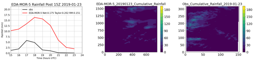
Figure 22 Surface rain rate skill scores and diagnostic maps of cumulative rainfall. The results are shown for an LES run using EDA05 forcing and Morrison microphysics for the case on 1 January 2019. The left-most plot shows the comparison of the region-averaged observed and simulated rain rate (mm h-1) with the Taylor-based skill scores given in the legend. To the right are the cumulative rainfall amounts in mm from the simulation (center image) and from observations (right image).
Sounding and Hodograph Diagnostic Plots
Diagnostic plots (without skill scores) are available that compare the simulations to the profiles available from the ARM-launched sondes. ARM had two sounding locations: one at the AMF central site just east of the Sierras de Córdoba mountain range, and an upstream ancillary site west of the mountain range at Villa Dolores. Sondes were launched at the AMF site every six hours starting at 0 UTC, and at the ancillary site they were launched every 12 hours starting at 0 UTC. An example of the comparison is given in Figure 23. We note that the NSF-led RELAMPAGO field campaign also launched numerous sondes during their operations, which users can download and use for their own model evaluation as well.
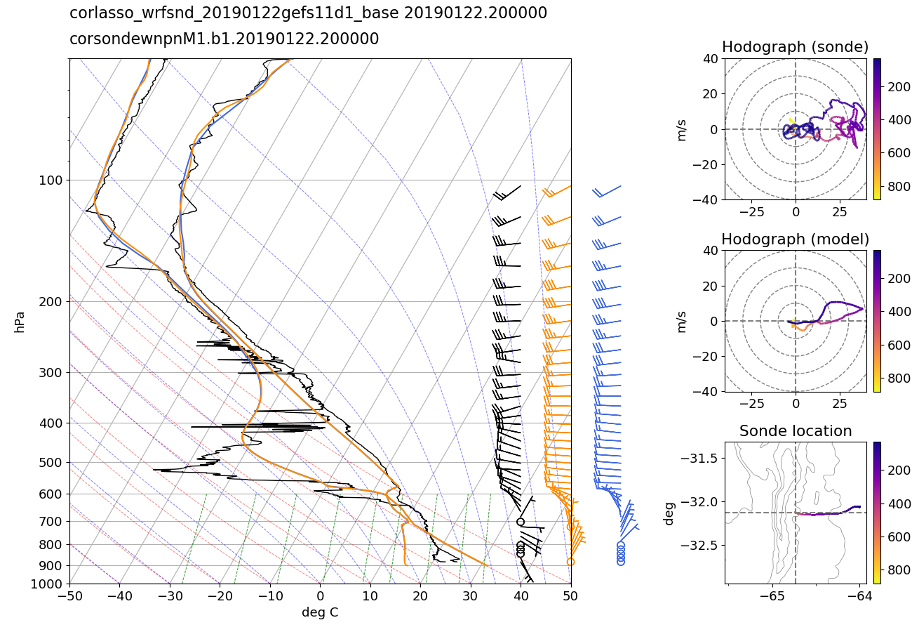
Figure 23 Example of the sounding and hodograph plots. Results are shown for a mesoscale simulation on 22 January 2019 that used the GEFS11 forcing and Thompson microphysics. This sonde was launched from the AMF central site. The black profile is from the radiosonde. The orange and blue profiles are from the simulation, with the orange profile sampling the model along the balloon track and the blue profile sampling directly over the balloon launch location. The balloon track is shown on the map in the bottom-right panel. The colors in the hodograph and map indicate the elevation of the sonde balloon in pressure coordinates (hPa).