Software for LASSO-CACTI

LASSO-CACTI Code Repositories

Codes used to pre-process data, run the WRF simulations, and work with the model output are available in git repositories at https://code.arm.gov/lasso/lasso-cacti. Table 37 lists the primary repositories of interest to users. Additional repositories are available on the site with code used more specifically for preparing and staging data for ARM infrastructure purposes.

Table 37 Useful code repositories available at https://code.arm.gov/lasso/lasso-cacti.

Name	Description
automate_meso	A series of scripts used to simplify running the mesoscale ensembles
cacti_notebook_library	Library of example Jupyter notebooks for LASSO-CACTI, described below
lasso-wps-cacti	WPS code modified for LASSO-CACTI
lasso-wrf-cacti	WRF code modified for LASSO-CACTI
subsetwrf	Python code to subset variables and add additional diagnostics from the raw wrfout files, described below

Sample Jupyter Notebooks

A selection of sample Jupyter notebooks are available to help users work with LASSO-CACTI data. These notebooks serve as a starting point which users can customize to meet various needs. Examples of these notebooks include versions to plot skew-T log-P diagrams, cross-sections through the model domain, and contour plots on maps.

The library of sample notebooks is pre-staged on the global filesystem at /gpfs/wolf/atm123/world-shared/cacti/beta_release/notebooks and can also be found in the https://code.arm.gov/lasso/lasso-cacti/cacti_notebook_library repository. The available notebooks are listed in Table 38.

The initial notebook library is provided by the LASSO team. We hope that over time this software library will grow to include community contributions to demonstrate additional plotting approaches and processing workflows, both using Jupyter and code directly run from the command line. Interested contributors can contact lasso@arm.gov for more information.

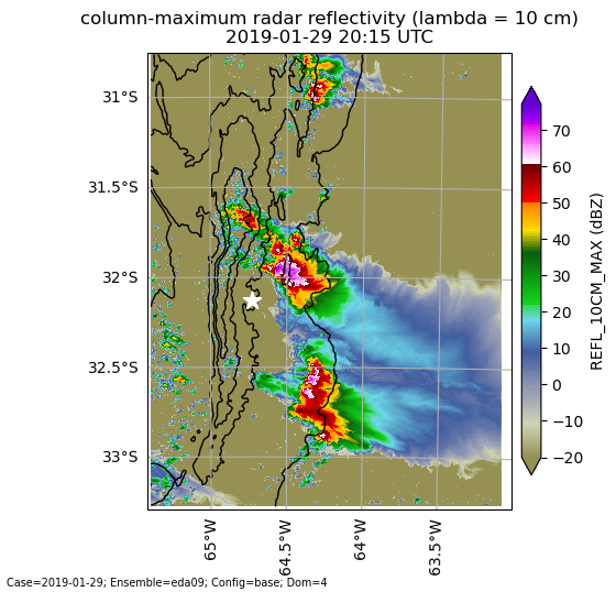
Figure 29 Simulated column-maximum reflectivity (dBZ) from domain D4 of the EDA05 base simulation at 29-Jan-2019 20:15 UTC. Code to generate this plot is in the plot_map_scalar.ipynb notebook. Black contours show the terrain at 500, 1000, 1500, and 2000 meters. The white star indicates the AMF location. Code to reproduce this plot is in plot_map_scalar.ipynb.

Table 38 Sample Jupyter notebooks available with LASSO-CACTI.

Filename	Description
plot_map_scalar.ipynb	Shows various ways to plot scalar variables on a map using LASSO-CACTI subset files
plot_map_vectors.ipynb	Shows various ways to plot wind vectors from the LASSO-CACTI subset files
plot_snd.ipynb	Shows how to use metpy to plot soundings and hodographs comparing data from the LASSO-CACTI subset files with observed ARM soundings
plot_snd_fromwrfout.ipynb	Similar to plot_snd.ipynb, but uses raw wrfout files for input
plot_timeseries.ipynb	Shows how to connect subset files in time and plot a time series at a given location using xarray
plot_xsec_scalar.ipynb	Shows examples of different ways to plot X-Z cross sections of LASSO-CACTI subset data

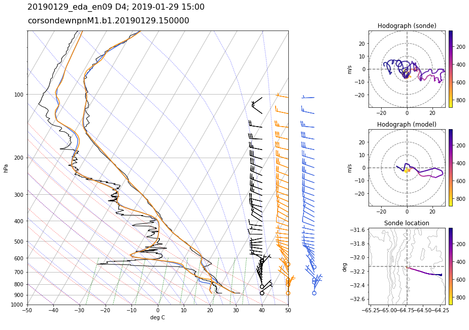
Figure 30 Skew-T log-P and hodograph plots from the ARM radiosonde and LASSO-CACTI WRF simulation on 29-Jan-2019 15 UTC from ensemble member EDA09, domain D4. For the skew-T, black=observed profile, orange=WRF profile following sonde track, blue=WRF profile at fixed launch location. Colors on the hodographs and sonde location plots show the height of the sonde over time in pressure (hPa). The sonde location plot shows the spatial path of the sonde with height contours in gray. Code to reproduce this plot is in plot_snd.ipynb.

Subset WRF Tool

The subsetwrf tool, available at https://code.arm.gov/lasso/lasso-cacti/subsetwrf, automates extraction of selected variables from the raw WRF output. This software is what produced the various “subset” file types available with LASSO-CACTI. Users preferring a different grouping of subsetted variables than those already available can run subsetwrf themselves to optimize their particular workflows. Note that this will require first downloading the full raw WRF output files, but it can make subsequent analyses easier by reducing the file sizes for plotting, etc.

The core of this software library is subsetwrf.py, which is controlled through a combination of command line arguments and an input YAML file that contains the list of variables to extract from the wrfout files. Optionally, variables can be interpolated from raw model levels to levels defined by pressure, height above ground, or height above mean sea level.

The git repository contains the YAML files for the variable groupings used with LASSO-CACTI. For example, met.yaml, metOnHagl.yaml, metOnHamsl.yaml, and metOnP.yaml define the particular variable groupings for the meteorological state variables on the various vertical-level options.

Specifics regarding the command line arguments for subsetwrf.py can be found in the README file.

Note that subsetwrf uses a combination of Python and Fortran code. One must first run numpy.f2py prior to running subsetwrf.py. The specific command is

python -m numpy.f2py -c module_diag_functions.f90 -m diag_functions --f90flags='-fopenmp' -lgomp

Also, since subsetwrf.py is often applied across many WRF output files, an additional tool called generate_slurm_task_list.py is provided that generates the commands necessary to submit a chain of subsetwrf.py commands using a Slurm job array. This permits users to parallelize the subsetting process across a pre-selected number of compute nodes. By setting the maximum permitted node count, users can control how much of the cluster is used at a time, thus ensuring sufficient nodes are left to share with other users.

Control of the Slurm task count is done by adjusting the --array option within the Slurm submission script produced by generate_slurm_task_list.py. The general syntax of this command is

# SLURM --array=<start>-<end>%<max tasks>

where the “start” and “end” integers define the first and last task numbers to process from the input task file, and “max tasks” is the maximum number of tasks to permit at a given time.

Instructions for running generate_slurm_task_list.py can be found at the top of the file. Most inputs are controlled via an input YAML file that identifies which WRF output files to subset.