Input Data Sets

Running WRF requires a range of input data sets, which are described in this section.

Soil Initial Conditions

The LASSO team generated initial conditions for the soil (moisture and temperature profiles) using the WRF-Hydro model (v5.1.2, https://ral.ucar.edu/projects/wrf_hydro; [Gochis et al., 2021]), downloaded from Github (https://github.com/NCAR/wrf_hydro_nwm_public/). The WRF-Hydro model has been configured to use the Noah-MP land surface model without any surface or subsurface routing. For each WRF mesoscale domain, we run a single, continuous WRF-Hydro simulation from 1 August 2018 through 21 March 2019, which allows the soil to spin up sufficiently prior to the first LASSO-CACTI case near the end of October 2018. The initial conditions and meteorological forcings for WRF-Hydro are from ERA5-land (https://www.ecmwf.int/en/era5-land) and interpolated to the resolution we need using a modified version of the WRF-Hydro Meteorological Forcing Engine (MFE) downloaded from Github (https://github.com/NCAR/WrfHydroForcing).

For evaluation, we performed a simple point-by-point comparison of the WRF-Hydro model output with in situ observations from the RELAMPAGO surface stations (11 stations in total) downloaded from NCAR (https://data.eol.ucar.edu/dataset/553.034). We find that the WRF-Hydro simulations provide more realistic estimates of soil moisture than ERA5-land for almost all stations.

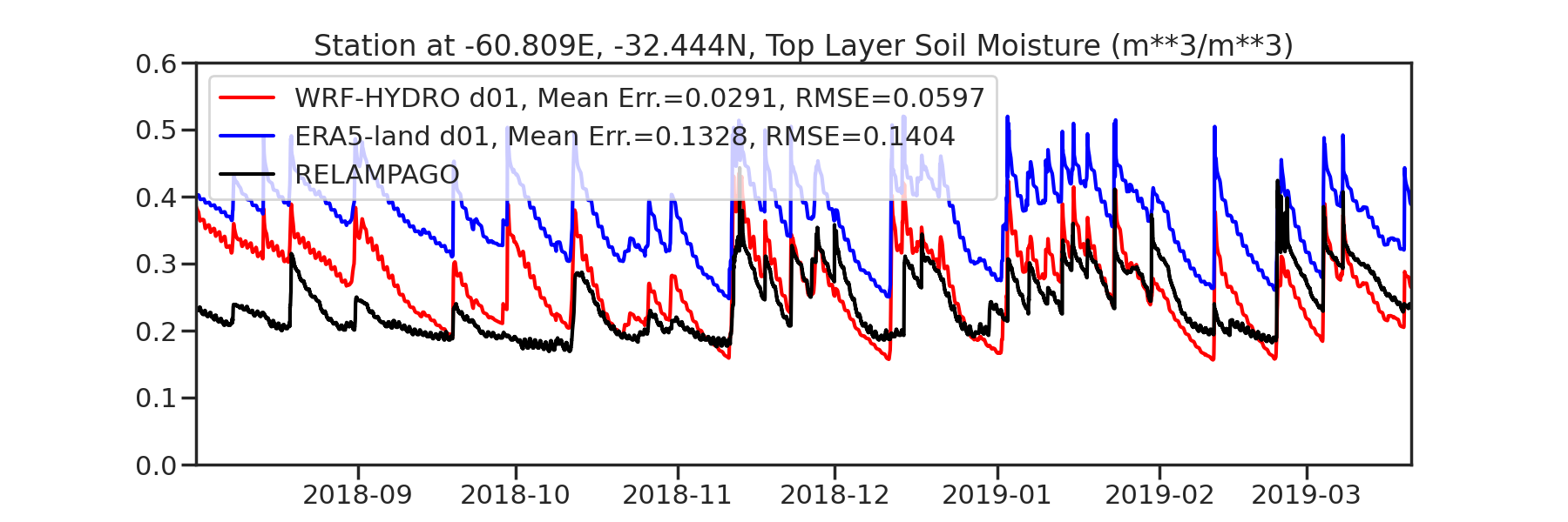
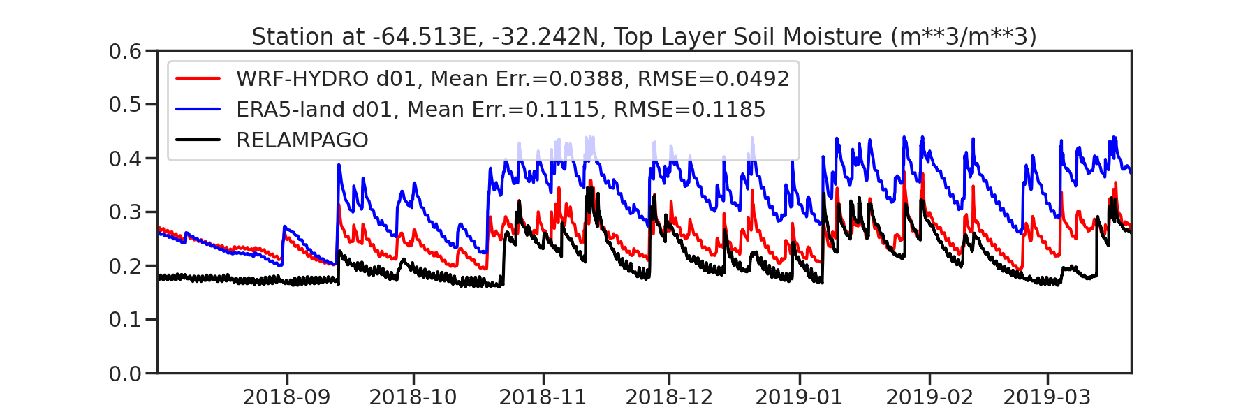
Figure 13 Time series of top-layer soil moisture (m³m⁻³) from ERA5-Land (0–7 cm), WRF-Hydro simulation ((0–10 cm, domain 1, 7.5-km horizontal grid spacing) and RELAMPAGO surface station observation (5-cm probe depth), for two stations, one (Gaboto, 19-m elevation) on the eastern edge of domain 1 (upper panel), the other (Quillinzo, 546-m elevation) near the center (lower panel).

The full WRF-Hydro simulation will be available as a sidecar product alongside the LASSO-CACTI atmospheric simulations. The WRF-Hydro simulation is referred to as the corlasso_wrfhydro data set within LASSO-CACTI. Users will be able to download all or part of corlasso_wrfhydro from the Bundle Browser. Contact lasso@arm.gov for access before the formal release.

Unlike the atmospheric simulations, which are episodic based on case date, corlasso_wrfhydro is continuous as a single simulation for the entire period. So, it can be used to initialize other case dates beyond what is already available for the mesoscale and LES simulations. It can also provide a spatial representation of the soil state throughout the CACTI campaign, with the caveat that this is a fully model-based product. Therefore, users need to approach its use accordingly.

Topography Data for WRF

The default topography data in WRF is available at 30-arcsecond (nominally 926 m at the equator) grid spacing. This is sufficient for most modeling, but at LES scales one can benefit from using higher-resolution data, particularly in complex topography as exists in the Sierras de Córdoba region of Argentina. For LASSO-CACTI we substituted DEM data from the Multi-Error-Removed Improved-Terrain Digital Elevation Map (MERIT DEM; [Yamazaki et al., 2017]) data set in place of the default WRF topography data. The raw MERIT data has a grid spacing of 3 arcseconds (93 m at the equator), which we smooth with a 1-km-scale filter using software from Branko Kosovic, NCAR, to improve model stability. While the smoothing removes some of the high-resolution details, the higher-resolution grid spacing permits more accurate sampling onto the LES grid.

For those interested in reproducing the processing of the DEM data, the workflow is as follows:

• Obtain the DEM data for the region of interest from http://hydro.iis.u-tokyo.ac.jp/~yamadai/MERIT_DEM/

• Use the convert_geotiff software from https://github.com/openwfm/convert_geotiff to convert the data from GeoTIFF to the format required for WRF’s geogrid.

• Manually adjust the index file for the resulting data tiles to compensate for any rounding errors due to that file being in single precision. The high-resolution data is of sufficient detail that double precision is required to fully capture the data accurately. For LASSO-CACTI, we find that a small adjustment is necessary, which can be identified by plotting known elevations against the resulting data.

• Place the new topography data tiles in a directory within the WRF_GEOG directory, which we call topo_merit_3s.

• Modify the GEOGRID.TBL file to include the new data set. Add the following lines to the HGT_M variable:

interp_option = topo_merit_3s:average_gcell(4.0)+four_pt+average_4pt
rel_path = topo_merit_3s:topo_merit_3s/

• Indicate in the namelist.wps file that the topo_merit_3s data is to be used when available:

geog_data_res = 'topo_merit_3s+9s+15s+gmted2010_30s+default',
                'topo_merit_3s+9s+15s+gmted2010_30s+default',
                'topo_merit_3s+9s+15s+gmted2010_30s+default',
                'topo_merit_3s+9s+15s+gmted2010_30s+default'

• Generate domains and apply terrain smoothing. We took the approach of 1) generating a geogrid file with a high-resolution topography data for a large domain, 2) applying smoothing, and then 3) sampling the topography data for each simulation domain. This is expected to result in smoother transitions at the domain boundaries compared to the approach of directly smoothing the topography data in actual simulation domains.

  • Run WRF’s geogrid.exe to generate a geogrid file covering the outermost D01 domain with the resolution of the innermost D04 domain (100 m).

  • Apply smoothing to the terrain data with 1-km scale using code from https://github.com/NCAR/WPS-GEO-LocalFilter developed by Branko Kosovic.

  • Run WRF’s geogrid.exe to generate geogrid files corresponding to actual simulation domains (D01, D02, D03, D04).

  • Replace terrain data in the D01-D04 geogrid files with those sampled from the smoothed high-resolution terrain data.

Meteorological Initial and Boundary Conditions for Mesoscale Ensembles

A selection of global analyses and reanalyses have been used to generate an ensemble of initial and boundary conditions for the LASSO-CACTI mesoscale simulations. Each of the input data sets is processed through the WRF Preprocessing System (WPS) and then used to initialize and drive the LASSO-CACTI D1 and D2 domains with 7.5-km and 2.5-km grid spacings, respectively. Table 15 lists general details for each data set. The resulting input options for LASSO-CACTI sums to 33 ensemble members per case date, with a small number of cases having missing or corrupt data for some members, resulting in slightly fewer members. The known bad ensemble members excluded from LASSO-CACTI are listed in Table 16.

Table 15 Meteorological data used for initial and boundary conditions of the mesoscale domains.

Source Name	# of Ensemble Members	Grid Spacing	Data Frequency	Source Archive	Reference
ECMWF Reanalysis V5 (ERA5)	1	0.25°	3 hours	https://cds.climate.copernicus.eu/#!/home	Hersbach et al. [2020]
ECMWF Ensemble of Data Assimilations (EDA)	10	0.5°	3 hours	https://cds.climate.copernicus.eu/#!/home	Isaksen et al. [2010]
Global Data Assimilation System Final Analysis (FNL)	1	0.25°	6 hours	https://rda.ucar.edu/datasets/ds083.3	NCEP et al. [2015]
Global Ensemble Forecast System (GEFS)	21	1°	6 hours	https://www.ncei.noaa.gov/products/weather-climate-models/global-ensemble-forecast	Zhou et al. [2017]

Processing of these different data sets generally follows the traditional handling of input data as described in the WRF documentation [Wang et al., 2019]. This involves converting the raw GRIB-formatted data (details for GRIB1 and GRIB2) into WRF’s “intermediate” format using the ungrib.exe program followed by metgrid.exe to interpolate data from the input grid to the WRF domain grids.

Note that the two ECMWF data sets for LASSO-CACTI are used on raw model levels. This requires extra steps in the WPS workflow to calculate the pressure levels, which is also described in the WRF documentation. One difference from the standard workflow is that the original 137 ERA5 levels are thinned to 89 levels using WPS’s mod_levs.exe program. We find that the full-resolution data combined with the large number of grid cells in D4 led to processing errors if we use more than 89 levels. The culled levels generally come from the stratosphere and two levels from the troposphere. The resulting vertical resolution in the stratosphere reduces to approximately that of the GEFS data. Specifically, the retained levels selected in namelist.wps are set via the following namelist block:

&mod_levs
press_pa = 200100,29,36,40,47,49,51,53,54,55,56,57,58,59,60,61,62,63,64,65,66,67,68,69,70,71,72,73,74,75,76,77,78,79,80,81,82,83,84,85,87,88,89,90,91,93,94,95,96,97,98,99,100,101,102,103,104,105,106,107,108,109,110,111,112,113,114,115,116,117,118,119,120,121,122,123,124,125,126,127,128,129,130,131,132,133,134,135,136,137
/

Table 16 Bad input ensemble members due to input source data.

Case Date	Source Name	Ensemble #(s)
19-Dec-2018	GEFS	6
29-Jan-2019	GEFS	6, 8, 13, 16, 17
23-Feb-2019	FNL	N/A (deterministic)
15-Mar-2019	FNL	N/A (deterministic)

One namelist.input setting adjusted to improve the simulations is increasing the width of the lateral boundary relaxation region from the default of 4 grid cells to 9. This is done by setting spec_bdy_width=10 in conjunction with specified=1 (the default value for the latter). This better constrains the outermost domain, D1, to the forcing data and provides for a cleaner transition region around the lateral boundary of this domain.

Aerosol Fields for Thompson Microphysics

LASSO-CACTI uses the aerosol-aware version of Thompson-Eidhammer microphysics [Thompson and Eidhammer, 2014, Thompson et al., 2008, Thompson et al., 2004]. Therefore, a background aerosol field and surface emissions are required for the aerosol particles. The Thompson-Eidhammer parameterization simplifies these down to two aerosol categories, which are named the “water friendly” aerosol and the “ice friendly” aerosol. A climatological value could be used, but this would not be particularly representative of the day-to-day conditions around the Sierras de Córdoba due to synoptic variability combined with complex topography. Therefore, aerosol information is obtained from the Goddard Earth Observing System Version 5 (GEOS-5) model [Rienecker et al., 2008].

Juliano et al. [2022] describes the mapping of species-specific GEOS-5 aerosol to the parameterized “friendly” aerosol categories. The algorithms and software used to implement this mapping were developed for the WRF-Solar variant of WRF [Jimenez et al., 2016], and portions of the WRF-Solar code are merged into lasso-wps-cacti and lasso-wrf-cacti, the LASSO versions of WPS and WRF. We are grateful to Tim Juliano and Pedro Jimenez, both from NCAR, for sharing code and assistance in merging it into the LASSO workflow.

The GEOS-5 data are obtained from https://portal.nccs.nasa.gov/datashare/gmao/geos-fp/das with a frequency of three hours. They are then converted to WRF’s intermediate format so they can be ingested by metgrid.exe when horizontally interpolating input data to the WRF grids. Users interested in downloading GEOS-5 aerosol information for other days or for altered model configurations should look at the create_geos_inter.py file within lasso-wps-cacti repository. The create_geos_inter.py script, located in the util directory, automates the workflow described in this paragraph for obtaining the aerosol data and converting them into the intermediate file format.