Modeling Methodology

WPS and WRF Code Used for LASSO-CACTI

LASSO-CACTI uses a customized version of the WRF model for simulating both the mesoscale and LES-scale simulations. The customizations generally add features needed for the LASSO application as opposed to fundamentally altering the model. Thus, the model behavior should follow the expectations of a typical WRF configuration.

The WRF workflow consists of two primary components, the WRF Preprocessing System (WPS) and the actual WRF atmospheric model. Both have added features for LASSO-CACTI. The code repository for LASSO-CACTI-WPS is at https://code.arm.gov/lasso/lasso-cacti/lasso-wps-cacti and LASSO-CACTI-WRF is at https://code.arm.gov/lasso/lasso-cacti/lasso-wrf-cacti. LASSO-CACTI-WPS is based on NCAR’s v4.3 code at https://github.com/wrf-model/WPS; LASSO-CACTI-WRF is based on NCAR’s v4.3.1 code at https://github.com/wrf-model/WRF.

The primary modifications to these codes include:

1. Code from the WRF-Solar project [Jimenez et al., 2016] has been incorporated to enable use of aerosol data from the global Goddard Earth Observing System Version 5 (GEOS-5) model to inform aerosol inputs for the Thompson microphysics parameterization. The species-specific aerosol information is mapped to the “water friendly” and “ice friendly” aerosol proxies used by Thompson as described in Juliano et al. [2022]. This entails changes to WPS for interpolating the GEOS5 data onto WRF grids as well as the associated code changes in WRF to use the aerosol information. We are grateful to Tim Juliano and Pedro Jimenez from NCAR for sharing code and assistance in merging it into the LASSO workflow.

2. Four inert tracers have been added to WRF to assist with feature tracking, examining flow characteristics, and other applications. These tracers are:

• Tracer 1: a conservative scalar initialized to have the value of the height above mean sea level for each grid point.

• Tracer 2: a conservative scalar initialized to have the value of the height above the surface for each grid point.

• Tracer 3: a unitless scalar (with zero initial concentration) that is emitted at the surface with a flux that is constant in both time and space, and decays with a time scale of 30 minutes.

• Tracer 4: a conservative “PBL” tracer that is initialized at 14 UTC after model spin up. It is initialized to a value of 1 for vertical levels below 1 km above the surface and 0 above that.

Note that the tracers are all initialized at the run start time except for Tracer 4, which is initialized 14 UTC to allow the boundary layer to spin up first.

3. The netCDF output format has been changed from CDF2 to CDF5 when not using the HDF5-based format tied to netCDF4, e.g., when using pnetcdf. This is required to accommodate the innermost WRF grid, which for LASSO-CACTI has too many grid cells to work with the CDF2 format. These code changes are based on Schwitalla et al. [2020].

4. Several additional diagnostic outputs have been added to WRF. These primarily consist of radiation fluxes and tendencies, convection parameterization tendencies, and microphysics process rates. Many of the additional microphysics process rates have been ported from diagnostics developed for the MC3E Intercomparison project [Fan et al., 2017]; specifics can be found in the code modifications to module_mp_thompson.F and related files in the lasso-wrf-cacti repository.

WRF Domain Configuration

As noted earlier, a two-stage approach is used for LASSO-CACTI that separates the mesoscale simulations from the finer-resolution LES simulations. This is accomplished with a downscaling workflow using the nesting capabilities in WRF such that two mesoscale domains are run with online, one-way nesting for the mesoscale simulations (7.5- and 2.5-km grid spacing), followed by an additional two domains that are run using online, one-way nesting for the LES (500- and 100-m grid spacing). These two pairs of domains were connected using the NDOWN software to convert output from the ∆x=2.5-km domain for use as input to the ∆x=500-m domain. This allows for clean handling of the separation between using a PBL parameterization for the two outer domains versus a subgrid-scale scheme for the inner two domains. The domain locations are shown in Figure 12. Note that we refer to the two mesoscale domains as D1 and D2 and the LES domains as D3 and D4.

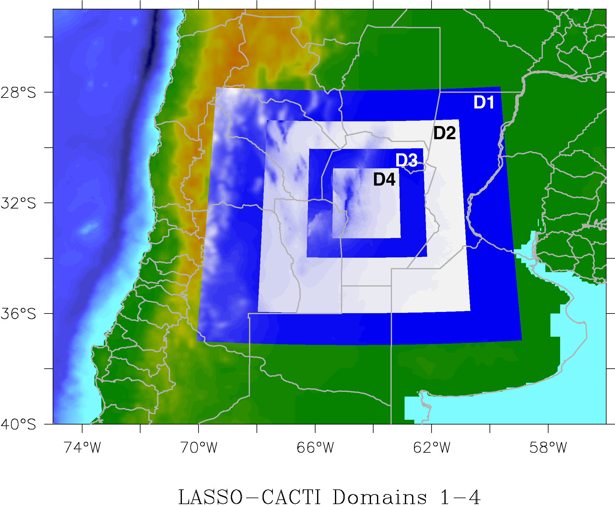
Figure 12 Locations of the four WRF domains. The two mesoscale domains are D1 and D2 with grid spacings of 7.5 and 2.5 km, respectively. The two LES domains are D3 and D4 with grid spacings of 500 and 100 m, respectively. The background shading is based on terrain height.

Each of the four WRF domains is roughly centered on the ARM Mobile Facility (AMF) location but with an eastward offset to permit convection to develop downwind of the site. Additional area is also included to the south for domains 1 and 2 because that region has large storm development that in some cases affects convection near the AMF.

Note that the downscaling approach to the LES grid spacings used in LASSO-CACTI significantly differs from the more traditional approach used in the LASSO shallow-convection scenario. The traditional approach uses doubly periodic lateral boundaries with a domain-average large-scale forcing tendency. In contrast, the downscaling approach uses spatially and temporally varying lateral boundaries, which permits location-specific details to be conveyed across the boundaries. The outermost domain receives boundary information from an analysis or reanalysis product, whereas the inner domains receive their boundary information from their parent domain. This enables one to do real-world simulations of specific weather events tied to the actual topography and other surface conditions.

Table 12 shows the dimensions of the four domains. Even though the innermost domain is substantially smaller, it has many more grid points due to its higher resolution. All four domains use the same 149 vertical levels (e_vert=150) spaced using WRF’s built-in auto_levels_opt=2 option with max_dz=1000 m, dzbot=25 m, dzstretch_s=1.05, and dzstretch_u=1.05. Note that a tall model top is requested with p_top_requested=1100 Pa to account for the very tall convective clouds associated with some CACTI cases. Overall, this results in a vertical grid with about 25-m spacing at the surface, which stretches to about 120 m at 2 km, maximizes at about 305 m near 6.5 km, and then reaches another minimum grid spacing of 225 m at about 18 km. The Noah land model is used with the customary four soil levels.

Table 12 Domain specifics for WRF configuration.

Domain	Category	Grid Spacing (m)	nx	ny
D1	Mesoscale	7500	131	137
D2	Mesoscale	2500	259	307
D3	LES	500	751	866
D4	LES	100	2146	2776

WRF Physics and Dynamics Configuration

The physics configuration used in WRF roughly follows the “CONUS” physics suite predefined in WRF. CONUS serves as the starting point, which is modified to turn off parameterization of deep convection for domains D2, D3, and D4, and the Mellor-Yamada-Janjic boundary-layer parameterization is switched to the Deardorff SGS scheme for domains D3 and D4. Radiation is handled by the RRTM shortwave and longwave schemes, which are called every two minutes. The primary physics settings are shown in Table 13 with full detail in these representative namelists for the mesoscale and LES runs, namelist.input.meso and namelist.input.les, respectively.

Dynamics parameters are generally set with default settings appropriate for the given grid spacings. For example, the newer hybrid vertical coordinates are used in conjunction with the moist-potential temperature to achieve greater accuracy from the dynamics [Xiao et al., 2015]. One change to note is that monotonic advection is used for the moist, scalar, and tracer variables.

Table 13 Important physics parameterizations and dynamics settings used for LASSO-CACTI WRF simulations.

Physics Type / Parameter	Scheme Used	References
Microphysics	Aerosol-aware Thompson-Eidhammer	Thompson et al. [2004] Thompson et al. [2008] Thompson and Eidhammer [2014]
Deep convection	Modified Tiedtke (D1 only)	Tiedtke [1989] Zhang et al. [2011]
Longwave and shortwave radiation	Rapid Radiation Transfer Model for Global Climate Models (RRTMG) LW and SW	Mlawer et al. [1997] Clough et al. [2005] Iacono et al. [2008]
Boundary layer	Mellor Yamada Janjic (D1 and D2 only)	Janjić [2001]
Subgrid-scale turbulence	1.5 order TKE (D3 and D4 only)	Deardorff [1980]
Surface layer	Monin-Obukhov (Janjic)	Janjić [2019]
Land surface	Noah	Ek et al. [2003]
Gravity wave drag	D1 only	Hong et al. [2008]
Moist, scalar, and tracer advection	Monotonic	Wang et al. [2009]

Configuration Labels

The above description for the domains, physics, and dynamics choices reflect the base configuration available for almost all the LASSO-CACTI simulations. However, additional simulations have been performed with alternative configurations to examine model sensitivity or other factors. The most common variation is to substitute the Morrison microphysics scheme for Thompson. When a run differs from base, we identify this using a different “configuration label.” Users can select the particular configuration label when selecting simulations in the Bundle Browser, https://adc.arm.gov/lasso/#/cacti. Currently available configuration labels are listed in Table 14.

Generally, all runs use the same WRF namelist settings other than changes for the date. The exceptions are for differences between the configuration label options. The specific namelist used for each simulation is included in the tar file associated with the input data for the simulation, and that namelist can be used to verify the settings of a simulation.

Table 14 Available WRF model configurations used within LASSO-CACTI.

Configuration Label	Description
base	Base configuration used for most simulations
morr	Morrison microphysics substituted for Thompson
ysu	YSU boundary layer substituted for MYJ
ysumorr	1) YSU boundary layer substituted for MYJ 2) Morrison microphysics substituted for Thompson
dearck0p1	Deardorff parameter c_k=0.1 instead of 0.15
smagcs0p1	Smagorinsky with c_s=0.1 substituted for Deardorff SGS
smagcs0p3	Smagorinsky with c_s=0.3 substituted for Deardorff SGS